Scenario You are developing a new instructional unit that integrates science, math, and technology. As part of this unit, you are planning to have your students study weather and determine the significance of large quantities of data that are gathered around the clock. You will create an example of this project in Excel. Your finished Excel project will contain graphics, national and local weather data, charts, math functions, and links to websites.

• Create and save simple workbooks/worksheets as web pages in Microsoft Excel
• Insert a graphic into Excel
• Use cells in a column and row format to organize data
• Customize a spreadsheet layout
• Use textboxes for placing text
• Insert hyperlinks into spreadsheets
• Apply formatting commands to a spreadsheet
• Distinguish between .htm and .xls files and the _files folder
• Develop integrated content spreadsheets
• Perform calculations using formulas
• Integrate web data into Excel
• Convert raw data to aggregate data
• Create graphical representations of data with charts

• Microsoft Excel 2007/2010 (Windows)
• Internet search engine
• Sample completed problems: weather.htm or WeatherExampleFeb14_2013.htm

Concepts
Integrated curriculum :
A curriculum that is planned in a manner to enable learners to recognize how concepts, content, processes are interrelated, and seek connections between past, present, and future experiences/learning. For instance science and math may be combined into "smath."

Thematic teaching :
A means of integrating multiple disciplines beneath one large "umbrella" idea. The theme (space travel for instance) becomes the focus of students interest instead of participating in out of context problem solving events.

Spreadsheet:
Large visual representations of data in column and row format. It provides a means of calculating numbers along with determining and displaying (via graphs) inter-relationships among data. Although the spreadsheet concept goes back a couple centuries, the first electronic version was conceptualized in 1961.

Raw to aggregate data:
Data that has been pooled, but not processed can be put through a process of extraction, organization, and analysis to be transformed into useable/meaningful "information." This process can provide a real-life meaningful context to learning.

Procedures Getting Started

1. Launch Excel from the Start menu.
2. Save as weather.xlsx

Look at the figure below and compare it to your screen. The spreadsheet is divided into numbered rows and lettered columns. The intersection of a row and column is called a cell and the are referred to by their column and row. For example, the very first cell is called A1 for column A and row 1. At least one cell has a heavy line or highlight around it. We say that cell is "selected." That line is called the "cell pointer." The selected cell or range of cells is displayed in the active cell area. Whatever we type into a cell first appears in the Data Entry Line. There, we can edit the contents until we're ready to enter them into the spreadsheet. Press <Return> or <Enter> to enter the cell contents. Use the mouse, the tab key, or the arrows to move the cell pointer around the spreadsheet. Take a moment to learn these terms and practice moving around from cell to cell.

Obtain Data

1. Open the following National Weather Service address in Internet Explorer:
   
   
   
2. Under "United States Weather" click the drop-down menu and choose "Arizona," click "Go." Next, for the "most recently observed weather conditions" choose a region...click "Go." Select data starting with "Date" through the last line of numeric data (red arrow in graphic below). Copy.
   
   
   
3. Open a new Excel workbook. In cell A1 paste (Ctrl + V).
4. Delete columns of unneeded data as identified below in red
   
5. Type the labels in row 4. You will need to unmerge a few cells (click in the merged cells and choose "merge & center" to unmerge). Use Alt + Enter when you are typing in a cell to get the cursor to move to the next line down in the same cell. In the A column (cell A2) type the date in the 2-14-2013 format (use whatever day is listed in your data). Autofil down as far as that particular date goes. Repeat the process if the previous day's date is listed as well. I suggest moving the "Wind Chill"and "Wind" next to the "Air" temperature for future comparison. The best way to do this is to insert a new column (right-click on the column header letter, "G" for instance, and choose "insert column." Select the column you want to move by left-clicking on the column header letter "L" for instance...move the cursor down to the border of the selected data (4-way arrow), left-click & drag straight across to the new blank column you created previously, drop in the blank column.
   
   Format Data
   
6. Formatting column widths: move cursor between column letters...A & B for example....and double click to form fit the columns to the text. Select cells with labels and/or data to align them properly. Make headings bold. Change "Relative Humidity" data to whole numbers instead of percent to make it easier to represent in a chart (Hint: type 100 in a blank cell...click in that cell, copy, select the range of cells with the percentages, go to "Paste"..."Paste Special" and choose under Operation "Multiply" then "Ok." This should convert all of them to whole numbers. Be sure to put % in the heading label.
7. Insert a new column to the right of "Air" and enter "Air °C." Repeat this for "Wind Chill."
   Insert Function/Formula
   
8. In the two new columns create a simple formula that calculates the celsius equivalent of Fahrenheit. Convert Fahrenheit to Celsius: type =(5/9)*(G2-32) then press enter (G2 is the cell in the example that has the Fahrenheit data). Round to a whole number. Note: If there are cells with NA in them I suggest using an IF function at the beginning, =if(G2="NA",0,(5/9)*(G2-32). Auto-fill to the bottom.
   
9. Delete all rows of data EXCEPT the labels and all the rows pertaining to ONE 24-hour period (keep all February 12 for instance).
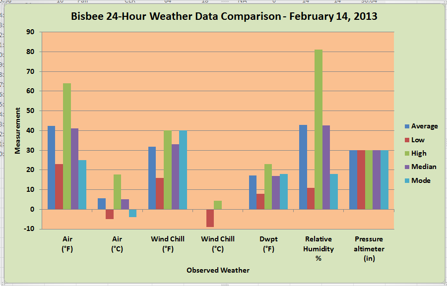
10. Enter labels for average, low, high, median, and mode at the bottom of your data like the example below. Enter functions in the first column referencing the appropriate cells above, select all 5 cells with the new functions and reduce/increase the decimal places to two, then auto-fill all 5 to the right (some column data type doesn't need these calculations as noted in the example below).
    
    Format Spreadsheet
    
11. Spend a bit of time formatting the spreadsheet with custom borders and shading as covered in previous Excel activities.
    Insert Chart as Object In
    
12. Create two charts: (a) a column chart based on average, low, high, median, and mode and the appropriate labels; (b) a line chart based on the time, air (F), and Dwpt (include the appropriate labels, but don't include the avg through mode). Format the charts to make them look nice as covered in previous assignments.
    
    
13. Adjust the properties of the chart by right clicking in various locations. Choose "format chart area" to adjust colors, font, etc. Choose "chart options" to adjust labels and legends.
14. Remove gridlines, adjust spreadsheet fonts, borders, fill, or anything else that will make the spreadsheet look optimum.
    

Raw data to aggregate data

1. Preview the U.S. Climate Normals (1971-2000) aggregate precipitation data. Notice the Arizona section on Pg. 6....a code is given (0299). Make note of this...it will be listed in the raw data you view next.
   
2. View the raw data for precipitation. You can also find it on the NOAA website (ASCII...month-year sequential values, .5Mb). Notice the txt file extension in your address bar. Also notice the column spacing between all the data except the top row. Save the file to your USB drive or the desktop. In excel click on your Sheet 2 tab. On the menu at the top click on "Data"..."Get External Data" group..."From Text" icon. Browse to the text file you just saved. Click "ok."
   
   
   
3. Notice the choose file type is showing "fixed width"...indicating that a column layout was detected in the text file. Click next...next...finish (accepting all the default settings). Click "Ok" accepting the setting "Existing worksheet."
   
   
4. Notice that the first row of text was not imported properly...it wasn't in corresponding columns.
   
5. Select cells A1 through H1...press the "delete" key to remove the cell entries (does not delete row, only text). In cell A1 type "Precipitation Totals By Month." Using skills in previous steps, clean-up the data/formatting...adjust column widths, etc. Insert a blank row above row 2 (select row 2...go to "Home" tab..."Cells" group..."Insert"..."Insert Sheet Rows").
6. Select Column "O"....delete. In Cell O3 type "Annual Precipitation." Right click over the top of the column heading letter "O"...choose "Column Width"....type in 20...click "ok."
   
   
   Sum Formula

1. Click in cell "O4" and type the formula "=sum(C4:N4)" (without the quotation marks) then press enter. Alternatively, you can click on FX on the formula bar and go through the step-by-step function procedures. You can also type =sum(  then use the mouse to click and drag the range of cells C4:N4 instead of typing them (or use the autosum key).
2. Click in cell "O4" again. Move cursor over the small black square (autofill handle)...either double click or press and hold the left mouse button...drag down to cell "O5113"
   
3. Freeze panes: In order to make the spreadsheet more user friendly....click in cell C4. Go to the "View" menu item..."Window" group...Freeze Panes. This will allow you to scroll the data without losing your column headings or left-hand row labels at the point indicated below. In order to unfreeze panes...go to "Window"..."Freeze Panes"..."Unfreeze Panes."
   
   
   Filter Data

1. Filter data: click in cell A3. Go to Data...and click on the "Filter" icon. This will make drop-down menus appear in row 3. click the drop-down in cell A3...uncheck "Select All"...scroll down put a check next to Arizona's code: 299 (as identified  in step 1 of the Raw data to aggregate data section above, but no zero shows in the dropdown). This will filter the data so that only the Arizona data is visible.
   
   
   3D Referencing

1. Go to Worksheet 3 and type in the text/data as indicated in the picture below (the top line is only in cell A1). Click in cell B3 and type the first part of the Average formula as indicated below. Once you have typed the opening parenthesis, you will see a message indicating the required series of numbers to average. With the mouse, click on the Worksheet 2 tab.
   
2. Scroll to the right so that the total column is near the year column. With the mouse, select the data in O74 to O83 (10 years of annual precipitation in the O column). Press enter. This automatically enters the data into your formula and takes you back to Worksheet 3. Repeat this for each block of 10 years in cells B4 to B9 of Worksheet 3.
   
   
   Logical Statements

1. IF Function: Excel has the unique capability to bring back or classify specific data according to criteria. It is important to place the data in a logical statement (true/false). Excel goes through the formula from the beginning...if it matches the indicated data as being true, it will not continue through the entire statement. In this example, we will enter an "IF" statement (used when there are 2 possibilities). Our criteria will be High Precipitation (H) and Low Precipitation (L).
2. In cell C3 we type the formula (alternatively you can select FX near the address bar), =if(B3>=13,"H","L") press enter. The formula is analyzing the data in cell B3 to determine which criteria it fits...it must be either at or above 13 to receive the "H", otherwise it is assigned "L." After pressing enter it should return an "H" in that cell. Click in the cell again...autofill the formula down to cell C9. *Note: no spaces between letters/characters of formula.
   
   
3. Nested IF (3 or more criteria): If we want to determine H, M, and L we can use a Nested-IF Statement. Always have 1 less IF than possibilities. Again in cell C3, type =if(B3>=14,"H",if(B3>=12,"M","L")) Be sure to have one closing parenthesis for each IF used in a statement. Notice that a 3rd number isn't needed...the way the formula reads, if the data doesn't match the first two criteria, it automatically has to be the last one. This is a logical statement (similar to other mathematical concepts) so it is important not to break the logic or mix > < symbols. *Note: if we wanted to bring back a number instead of a letter, we would not use quotation marks.
   
   
   Moving Data

1. Moving Data: Right click over the column heading B and choose "insert." Left click in cell D3 and select down to D9. Move your cursor over the black border of the selected area...you should see a 4-way arrow. Press and hold your left mouse button...drag to the left and drop it into B3 through B9.
   
   
   
   
   Chart as New Sheet

1. Create Chart (multiple labels): Select data in cells A3 to C9. Click on "Insert" on the menu at the top. Choose "Column"..."3D Column "3D Clustered Column." Enter titles and axis labels....remove legend. Right click in a blank area of the chart...choose "Move Chart." Select "as new sheet" then type a name in the box to the right (as indicated below). Click "finish."
   
   
   

Textbox/Autoshapes/Lines to Place Text or Highlight Specific Areas

1. Textboxes/autoshapes/Lines/WordArt can be used in Excel to place text or hyperlinks over the top of charts, other text, etc. You have the option of showing borders and background shading, or make them transparent.
2. Many of these features have similar procedures as in MS Word.
3. Click on "insert"...and you will notice many of the selections on the toolbar. After typing your text in the box, right-click on the border of the textbox and go to "Format Shape."
    

Rename Worksheets

1. Right click on any particular worksheet tab to rename, insert new, or delete. You can also click and drag a worksheet tab left or right to change the order. All worksheets need to be named, and blank worksheets deleted.
   
   

Inserting Hyperlinks

1. Surf the site to which you wish to link. In this example, we're going to create a link to http://weather.noaa.gov/
2. Place your cursor in the cell where you want the hyperlink located.
3. Type the phrase that will be the hyperlink, for this example, we'll use "National Weather Service " as the target phrase. Press enter.
4. Single left click in the cell where you typed the phrase to select the cell.
5. Choose Insert > Hyperlink
   
6. Type in the url http://weather.noaa.gov and click "ok
7. Check all your pages to make sure everything is in order. Scroll up to the top of every page. Click on the tab of the worksheet you want your viewer to see first (the last page viewed when you save will appear next time it is opened).
   
8. Save and upload in the appropriate D2L dropbox.

Note: Be sure to check over the TIP assignment criteria. You need to include one or more worksheets in this same file that includes standards (Science, Student Technology, and NETS*T), along with directions/comments pertaining to the manner in which this project would be used by students. Format all worksheets in a appealing manner.